Examples
Every script below runs offline in a few seconds on a CPU. They use datasets that ship with scikit-learn, or synthetic data, so nothing is downloaded. The outputs shown are what each script prints with the seeds it sets. Your numbers may differ slightly across PyTorch versions.
pip install "fannar[all]"
git clone https://github.com/FernandoCsm-Knight/Fannar.git && cd Fannar/examples
python tabular_wine.py
| script | module | model and data | what it shows |
|---|---|---|---|
quickstart_digits.py |
fannar.tabular |
MLP, digits as 64 features |
the full tour: report, plots, pairs, swap test |
tabular_wine.py |
fannar.tabular |
MLP, wine as a DataFrame |
pandas input, named classes, pairs, errors |
tree_wine.py |
fannar.tree |
decision tree, wine, text labels |
depths as layers, slack scale, a tree as the floor |
image_digits_cnn.py |
fannar.image |
CNN, digits as 8×8 images |
DataLoader input, energy map of one image |
text_keywords.py |
fannar.text |
small transformer, synthetic sentences | wrap_hf, automatic layers, energy per token |
custom_gram.py |
fannar |
no model | your own sources, kernels and Gram matrices |
A table, with pandas
tabular_wine.py trains a small MLP on the 13 chemical measurements of the wine dataset. It
passes the test DataFrame and a categorical Series straight to
TabularInterpreter:
y = pd.Series(pd.Categorical.from_codes(data.target, ["barolo", "grignolino", "barbera"]))
...
interp = TabularInterpreter(model, X_te, y_te, layers=["block1", "block2"], reference_model=initial)
interp.feature_names[:4]   # ['alcohol', 'malic_acid', 'ash', 'alcalinity_of_ash']
interp.class_names         # ['barolo', 'grignolino', 'barbera']
The pair explanation says what separates a wine from the nearest one that the model puts in another class. The values are in the standardised scale the model was trained on:
par (0, 69): grignolino x barbera
  alcohol                        i = -1.08  j = +0.72  parcela 54%
  color_intensity                i = -1.05  j = -0.26  parcela 14%
  flavanoids                     i = -0.28  j = -1.22  parcela 11%
explain_errors aggregates the same reading over the three test errors. Compare each feature's
share among the errors with its share in general. ash and magnesium weigh much more in the
mistakes (18% and 15%) than in the model's decisions overall (11% and 5%):
  proline                        parcela nos erros 26% (em geral 25%), primeiro em 33%
  ash                            parcela nos erros 18% (em geral 11%), primeiro em 33%
  alcohol                        parcela nos erros 17% (em geral 16%), primeiro em 33%
  magnesium                      parcela nos erros 15% (em geral 5%), primeiro em 0%
The swap test checks the ranking. Each method orders the features, the features are swapped one by one from \(x_i\) to \(x_j\), and a larger area means the prediction flips sooner. Here the method's order beats both the size of the difference and a random order:
The same table, with a tree
tree_wine.py fits a depth-4 DecisionTreeClassifier on the same data, with the labels as text.
TreeInterpreter maps them to tree.classes_ (sorted:
['barbera', 'barolo', 'grignolino']). It uses the training standard deviation as the slack
scale, and a tree fitted on shuffled labels as the floor:
shuffled = DecisionTreeClassifier(max_depth=4, random_state=0).fit(X_tr, rng.permutation(y_tr))
interp = TreeInterpreter(tree, X_te, y_te, X_train=X_tr, reference_model=shuffled)
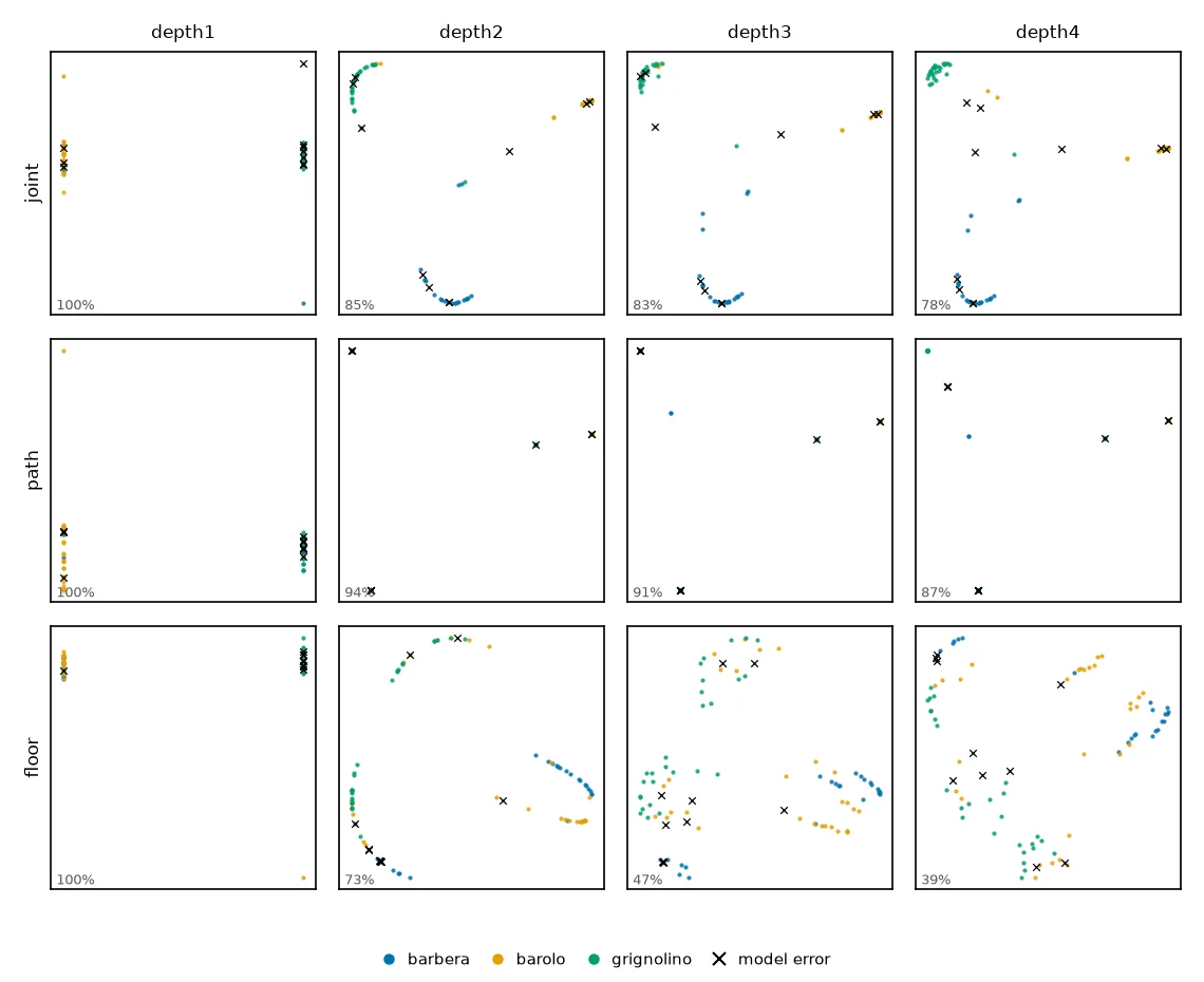
The pair explanation can be read per depth. The root splits on alcohol, and from depth 2 on
the decision moves to od280/od315_of_diluted_wines:
par (0, 83): grignolino x barbera
  od280/od315_of_diluted_wines   i =    2.57  j =    1.82  parcela 83%
  flavanoids                     i =    1.75  j =    0.48  parcela 17%
parcelas por profundidade (atributo principal): {'depth1': 'alcohol', 'depth2': 'od280/...', ...}
Images, and where the energy sits
image_digits_cnn.py reads the 8×8 digits as images (N, 1, 8, 8) and trains a three-block CNN
(97% test accuracy). ImageInterpreter receives the test DataLoader as it
is. Each block's output is pooled to a 4×4 grid, so conv3 has 32 channels × 16 positions per
object.
For one image, energy_map uses the positions as the objects:
emap = interp.energy_map(image, "conv2")                 # (8, 8)
interp.plot_energy_map(image, "conv2", image=image[0])
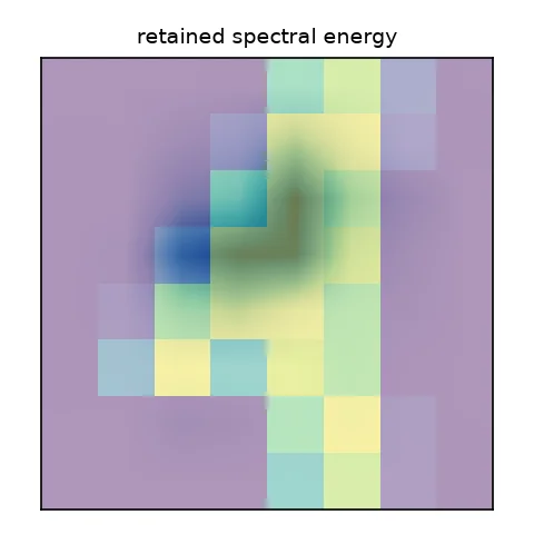
conv2 over a "1". The stroke covers
36% of the image and holds 72% of the energy.Text, layer by layer
text_keywords.py builds sentences of 8 to 16 tokens with padding. The class is a keyword placed
at a random position. The model mimics the Hugging Face interface (model(input_ids=...,
attention_mask=...) returns an object with .logits), so the script uses
wrap_hf as it would with a real model. It does not pass layers=, so the
three encoder blocks are found automatically.
The per-token energy shows how the information moves through the network. In the first two blocks the keyword is the token with the most energy. In the last block, attention has already spread it over every token:
frase 0: palavra-chave na posição 6 de 12; energia por token (normalizada):
  model.encoder.layer.0  [0.27 0.75 0.05 0.05 0.03 0.17 1.   0.32 0.31 0.07 0.05 0.55]
  model.encoder.layer.1  [0.22 0.55 0.16 0.06 0.03 0.21 1.   0.3  0.22 0.17 0.23 0.09]
  model.encoder.layer.2  [0.97 0.66 0.99 0.83 0.81 1.   0.99 0.97 0.92 0.95 0.94 0.91]

token de maior energia = palavra-chave (100 frases; ao acaso ~9%):
  model.encoder.layer.0  54%
  model.encoder.layer.1  66%
  model.encoder.layer.2  12%
Pick the layer for the question
Energy maps read the positions inside one layer. To see which tokens (or image regions) carry the information, look at the early and middle blocks. Near the output, attention and pooling have mixed the positions, and the map becomes uniform even when the model is right.